mobius2.html

Rubans de Moëbius tracés sur des cônes

I. Principe utilisé :

s:=4: S:=[s,0,0]:
n #--- le nombre de cones --------
Soit (H) la courbe du plan xh:=s*cos(Pi/n)^2 formant un "8" avec ymax= s/2*sin(2*Pi/n). Cette courbe peut être un "8" très approximatif : il suffit qu'il coupe perpendiculairement le plan Oxy aux points [xh,yh,0] et [xh,-yh,0]
Je considère le cône de sommet S de directrice (H) et une demi-bande de ce cône comprise entre les génératrices du plan xOy puis les transformés par rotations d'axe Oz d'angle 2*Pi/n

II. Le programme :

restart: with(plots):
ps:=proc(U,V) local u,v; u:=expand(U): v:=expand(V): add(u[i]*v[i],i=1..nops(u)): end:# produit scalaire
norm2:= proc(U) expand(U/sqrt(ps(U,U))): end:
rotz:=proc(t,pt) [pt[1]*cos(t)-pt[2]*sin(t),pt[1]*sin(t)+pt[2]*cos(t),pt[3]]: end:
tabcol:=[red,green,blue,cyan,magenta, khaki]:#---- rallonger pour n > 6 !!!
s:=4: S:=[s,0,0]: # --- le sommet du cone de base ----
n:=3 ; #--- le nombre de cones --------
xh:=s*cos(Pi/n)^2: yh:=s/2*sin(2*Pi/n):
#---- on pourrait simplifier un peu en mettant une bande de largeur non constante( enlever le norm2 )
bande:=proc(t,u) expand(H(t)+u*norm2(H(t)-S) ): end:
large:=0.5;

H:=proc(t) [xh,yh*cos(t)^3,yh*cos(t)^2*sin(t)]:end: inter1:=0..Pi/2: inter2:=Pi..3*Pi/2: inter0:=0..2*Pi:      #----- pour r=cos(t)^2
# H:=proc(t) [xh,yh*sin(t/2), sin(t)] end: inter1:=-Pi..Pi: inter0:=0..4*Pi:       #---- la lemniscate -----------
#--------- déformation qui conserve la perpendicularité des tangentes au plan xoy aux points[xh,yh,0] et [xh,-yh,0] ------
coX:=0.8; H:=t -> [xh+coX*cos(t/2)^2,yh*sin(t/2), sin(t)]; inter1:=-Pi..Pi: inter0:=0..4*Pi: ### déformation de la lemniscate (ou coX:=-0.5);
for i to n do:
      bande||i:= plot3d(rotz((i-1)*2*Pi/n,bande(t,u)),t=inter1 ,u=-large..large,grid=[30,200],color=tabcol[i],style=patchnogrid) :
     cone||i:= plot3d(rotz((i-1)*2*Pi/n,S+u*(H(t)-S)),t=inter1,u=0..1,grid=[20,3],color=tabcol[i],style=line) :
     ##### pour r=cos(t)^2 , ex\303\251cuter les 2 lignes suivantes sinon les annuler avec des "#" pour la lemniscate déformée ou non
     #bande||i:= bande||i, plot3d(rotz((i-1)*2*Pi/n,bande(t,u)),t=inter2 ,u=-large..large,grid=[30,200],color=tabcol[i],style=patchnogrid) :
     #cone||i:=cone||i ,plot3d(rotz((i-1)*2*Pi/n,S+u*(H(t)-S)),t=inter2,u=0..1,grid=[20,3],color=tabcol[i],style=line):
od:
display([
     tubeplot( H(t), t=inter0,radius=0.05,grid=[200,20],color=cyan,style=patchnogrid)
     , seq(cone||i ,i=1..n) , seq(bande||i ,i=1..n)
     ],scaling=constrained,axes=none,orientation=[30,40,0]);

directrice des cônes : lemniscate
trois cônes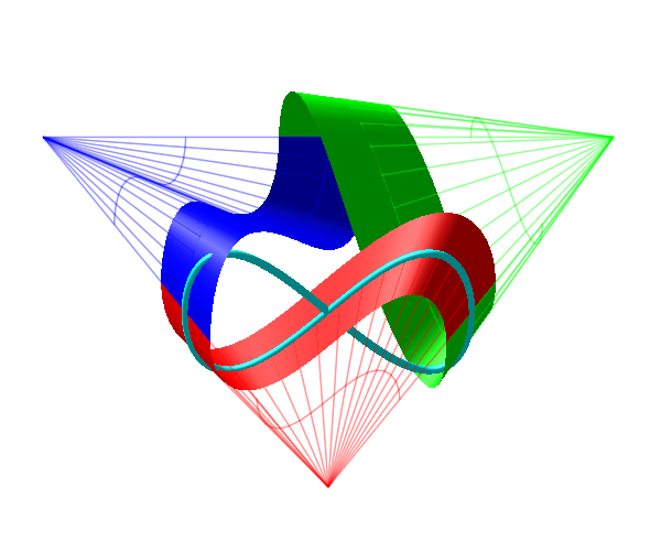	quatre cônes
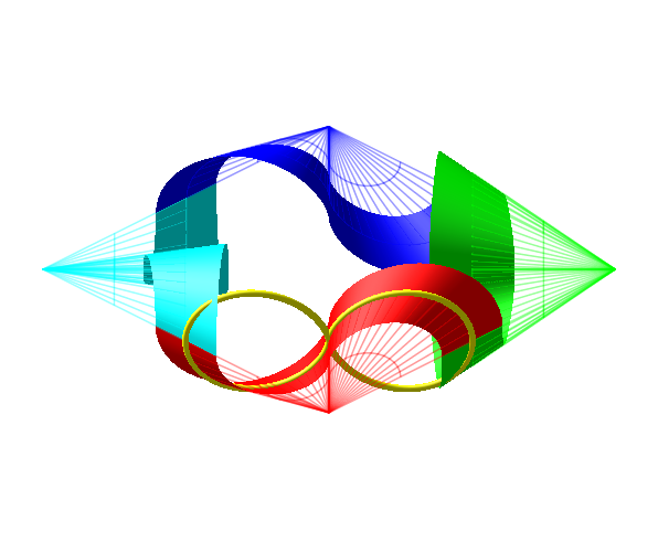
directrice des cônes : lemniscates déformées
coX=-0.5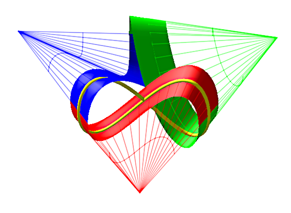 anaglyphe à regarder avec des lunettes rouge-cyan	coX=0.8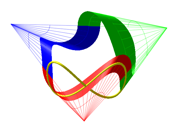 anaglyphe à regarder avec des lunettes rouge-cyan
directrice des cônes d'équation polaire : ro=cos(t)^2
trois cônes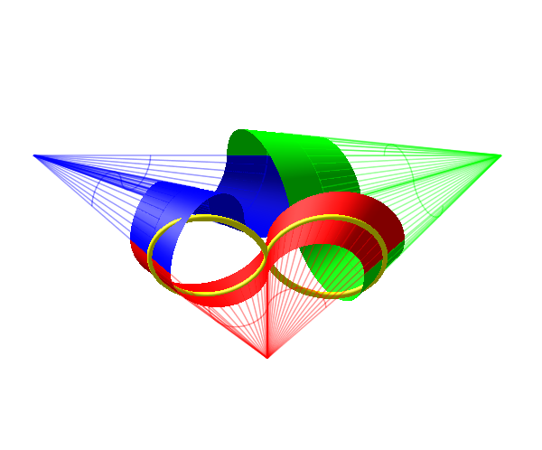	quatre cônes

III. Un ruban de Moëbius tracé sur deux cônes :

Le programme Maple

restart: with(plots):
ps:=proc(U,V) local u,v; u:=expand(U): v:=expand(V): add(u[i]*v[i],i=1..nops(u)): end:# produit scalaire
norm2:= U -> expand(U/sqrt(ps(U,U))):
r:=0.06:
#---- pour une bande de largeur non constante( enlever le norm2 )
bande:=(M,S,t,u) -> expand(M+u*norm2(M-S) ):
large:=0.7: s:=6.: R1,R2:=3,2:
M1:=[2*R1*cos(t)*cos(t),2*R1*cos(t)*sin(t),sin(t)]:
M2:=[-2*R2*cos(t)*cos(t),2*R2*cos(t)*sin(t),-sin(t)]:
S1:=[0,0,s]: cone1:= expand( S1+u*(M1-S1) ):
S2:=[0,0,0]: cone2:= expand( S2+u*(M2-S2) ):
inter:=-Pi/2..Pi/2: inter1:=0..Pi:
gr:=proc(lat,long)
display([ #mesaxes,
     tubeplot(bande(M1,S1,t,large),t=inter,radius=r,color=magenta,grid=[300,20],style=patchnogrid)
     ,tubeplot(bande(M1,S1,t,-large),t=inter,radius=r,color=magenta,grid=[300,20],style=patchnogrid)
     , tubeplot(bande(M2,S2,t,large),t=inter,radius=r,color=magenta,grid=[300,20],style=patchnogrid)
     ,tubeplot(bande(M2,S2,t,-large),t=inter,radius=r,color=magenta,grid=[300,20],style=patchnogrid)
     ,plot3d(cone1,t=inter,u=0..1,grid=[15,2],style=wireframe,color=red,thickness=3)
     , plot3d(cone2,t=inter,u=0..1,grid=[15,2],style=wireframe,color=blue,thickness=3)
     ,plot3d(bande(M1,S1,t,u),t=inter,u=-large..large,style=patchnogrid,color=green)
     ,plot3d(bande(M2,S2,t,u),t=inter,u=-large..large,style=patchnogrid,color=green)
    ],scaling=constrained,axes=none,orientation=[lat,long]):
end:
gr(30,90);